-
Notifications
You must be signed in to change notification settings - Fork 103
Introductory Tutorial: Part 3 Working with Labelled Data
This tutorial guide follows on from Part 1 and Part 2 of the introductory tutorial. We recommend starting doing those first, although this part is independent of the data and steps from Part 1 and 2.
→ If you are continuing from the previous example then use File > Close Data Book as before.
→ Go to File ⇒ import From Library.
→ Press on Load from R and select the package sjmisc.
→ Select the dataset called efc and press OK.
This loads a dataset that was originally in the statistics package SPSS. The data are a subset from a large European project on caring for the elderly. The full questionnaire is available here https://www.uke.de/extern/eurofamcare/documents/deliverables/cat_uk.pdf and Fig. 29 shows part of one page.
| Fig. 29 The survey on caring for the elderly by family members |
|---|
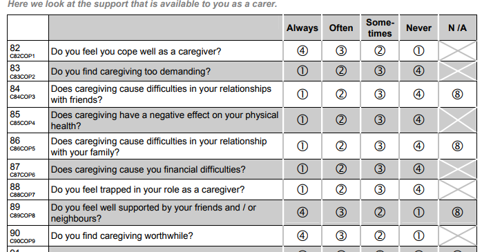 |
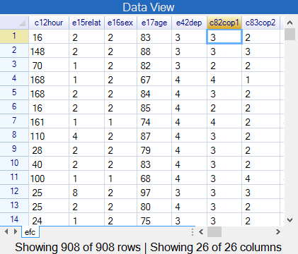
Fig. 30 shows a sample of the efc data in R-Instat. The names of the variables can be explained by comparison with Fig. 29. For example with the variable called c82cop1 the c signifies it is a question about the carer. The 82 is because it was question 82 in the questionnaire (Fig. 29) and cop1 is because it was the first question concerning coping. Hence, in Fig. 30, the name e17age is the age of the elderly person being cared for.
| Fig. 30 The efc data |
|---|
 |
More information is needed to be able to analyse this sort of data.
→ Choose View > Column Metadata or click on the icon with an i in the toolbar.
→ Edit the size of this window so it looks similar to Fig. 31.
| Fig. 31 The column metadata |
|---|
 |
Three items from Fig. 31 are as follows:
- The column variables also have a label as well as their name. Here the variable label is often the question in the questionnaire.
- All the columns are currently numeric.
- The categorical columns have a set of value labels, e.g. male = 1, female = 2.
In R and hence R-Instat the categorical columns are called factors.
These category columns are now to be changed into factors.
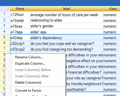
→ Go to the number 2, i.e. the left hand side of the second row (2 e15relat). Right-click and choose the option to Convert to Factor.
→ Repeat for all the category columns in the data set. You can mark multiple columns and convert them together, Fig. 32.
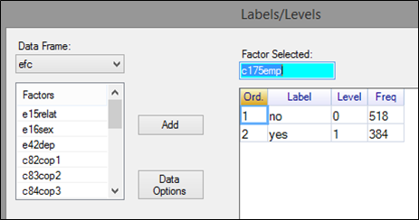
→ To understand factors in R-Instat a little more go to c175empl. Right-click on the number 18 and choose Levels/Labels. (If that option isn't enabled, then you haven't yet made that column into a factor, so do that first.) The result is shown in Fig. 32.
Notice that in Fig. 32 the numbers 0 and 1 are now called Levels, while no and yes are the Labels.
| Fig. 32. Converting columns into factors | The Levels/Labels dialogue |
|---|---|
 |
 |
These data are now ready to produce tables and graphs.
→ Close the Column metadata window, either by clicking on the icon in the toolbar, or from the View menu.
Start with 2 familiar dialogues from earlier, (Part 1 of the tutorial) as examples. So try:
→ Describe > One Variable > Summarise. Add all the columns and press OK.
→ Describe > One Variable > Graph. Choose the 9 columns from c82cop1 to c90cop9 and press OK.
Of course many analyses are possible. For example:
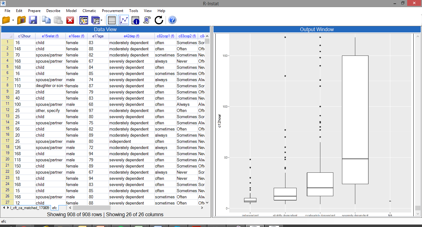
→ Use the Describe > Specific > Boxplot dialogue to produce the graph in Fig. 33 of the number of hours of care against the level of dependency.
| Fig. 33 The efc data with factors and boxplots |
|---|
 |
→ Before finishing, save the data (as shown in Part 2 of the tutorial) so the changes made above are kept, and the analyses could continue.
We are aiming for R-Instat to be accessible for beginners to statistics packages - but we assume that some of you may have some familiarity with R already. If not, then read, but omit this next task.
Go to View ⇒ Log Window, or press the log window icon on the toolbar. Copy the contents from the top to at least the first line that produces a graph. Then open R (or an R environment like RStudio) and paste the contents. You should get the same graph.
We are keen to encourage more experienced users to consider starting an analysis in R-Instat and finishing in R if they need to.
And, in addition, if things go wrong, you could try running the last commands in R, or send us the R code that was generated and didn't do what you wanted.
We provide a short description of where we are, menu by menu, and where we are heading in future versions.
a) File Menu You should be able to import data from a wide range of software, thanks to the rio R package, which is included for import and export. As shown above, we have now resolved how to import value labels from SPSS and Stata.
b) Different sized files. We are reasonably happy with the way long datasets are handled. In previous versions we faced speed issues and timeout errors which crashed R-Instat when using wide data sets. From Version 0.4 we have a substantial speed improvement for wide data sets. The introduction of a maximum columns to display has largely eliminated the occurrence of timeout crashes.
c) Spreadsheet Operations. We are fairly happy with the way the spreadsheet is working, including right click menus for users familiar with spreadsheet packages. The speed of refreshing the grid has significantly improved in this version. The spreadsheet is just a window onto your data, the default is to display only the first 1000 rows and 30 columns. This can be changed in the options. We would like to add paste facilities in the spreadsheet in future versions.
d) Prepare menu This is reasonably complete. There are good facilities for calculating new columns, for dealing with numeric and factor columns and also some for manipulating text and date columns. Merging and stacking facilities have been enhanced for this version. The dialogs for filtering, appending and unstacking data are also there, and will be enhanced further. We can now cope with labelled data (from SPSS or Stata, as described above), but have yet to add facilities for multiple missing value codes.
e) Prepare menu continued. We also have dialogs to manage keys and links between data frames and to manage R objects, e.g. graphs, models, and filters. These will be enhanced in later versions
f) Describe menu. You can summarise data quite well, and we now have some dialogs for tables with html output. We have spent a long time on graphics and have recently managed to implement facilities for the powerful themes component of ggplot2. This is still to be improved further as will other ggplot features, particularly for mapping and also adding to our list of available geoms.
g) Model menu. There is still a lot to be added here. We are happy with the structure of the menu, but improvements are needed for the output from the fitting, the range of models that can be processed, and also the facilities for choosing and using the models.
h) Climatic menu. A lot of work has been done on general facilities which relate to climatic data, such as handling dates and calculating and summarising columns. We have begun implementing tailored products, such as the inventory plot dialog, start of the rains and spells and many more are almost complete, such as extremes.
i) Procurement menu. This is for the analysis of procurement data to study corruption risks. It is currently tailored to the procurement data available in the R-Instat library. An expansion of these facilities will be in future versions.
j) Help menu. There is a lot to do here to have good help facilities. We will also add tooltips in dialogues. We have started to produce a series of short videos to explain a range of aspects concerning the use of R-Instat which will be available to users.
Now you are "on your own"! We hope you will enjoy playing with R-Instat and look forward to your reflections and feedback.