I finished my first half-marathon within 3 hours in 2019. It was a dreadful experience yet extremely rewarding. I did not train nor prepare myself for the marathon as it was a spontaneous decision, but I still managed to complete the 21km journey. Aside from the 'NEVER GIVE UP' spirit, I might have to thank my 'once in a while' outdoor cardio activities (i.e. mainly Running and Walking). Since 2014, I have been using a popular app called Runkeeper whenever I exercise outdoor. It is an excellent app that keeps track of your runs, goals and improvements. In this project, I would like to humbly present the analysis of my Runkeeper Fitness data and to provide an overview performance of my outdoor cardio activities. An unexpected insight will also be provided.
Runkeeper records a wide range of information describing user's activities, route, distance, duration, average pace, average speed, calories burned and average heart rate. An amazing key feature of Runkeeper is its excellent data export. User is allowed to download her/his data from the personal profile section.
- Obtain and review raw data
- Data Preprocessing
- Dealing with missing values
- Ploting running data
- Running statistics
- Did I reach my goal?
- Am I progressing?
- Detailed summary report
- Conclusion
import pandas as pd

#Name the dataset file and create a dataframe
runkeeper = pd.read_csv('/Users/lamyingxian/Dropbox/Data Science Course/Projects/My Cardio Activities - Runkeeper/cardioActivities.csv,parse_dates=True,index_col='Date')

#Brief look at the data
runkeeper.head()
👉 Since the console is not able to show all the 14 columns due to its limited space, I prefer to briefly look at the data in variable explorer.
#Summary of the data
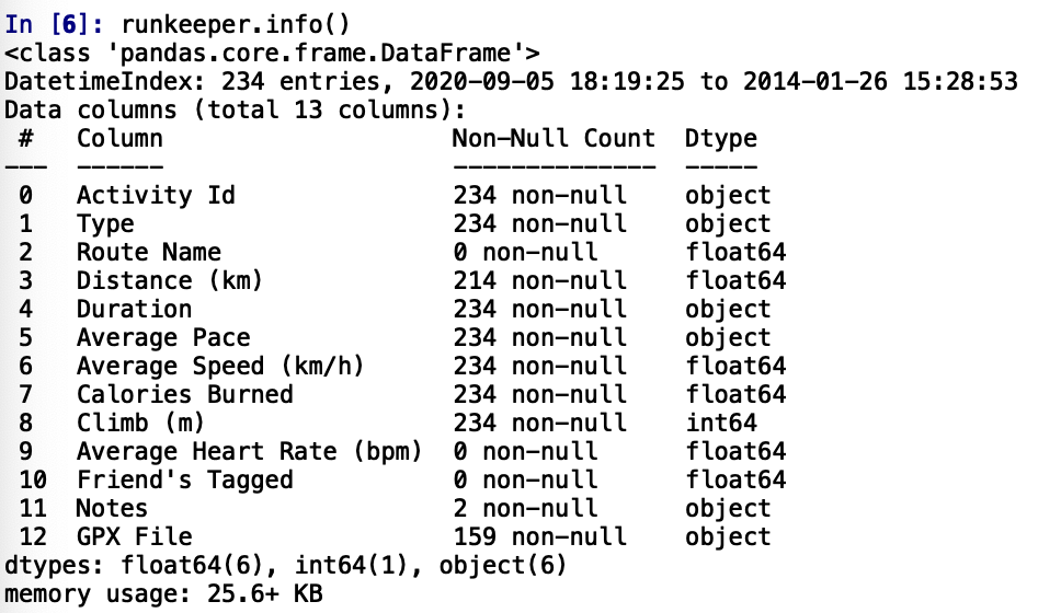
runkeeper.info()
👉 There are 234 data and 13 columns of data.
👉 'Non-Null Count' means number of items in the specific column that are not zero/empty. There are some missing values in 'Distance'. It will be explored deeper in Data Preprocessing.
👉 'Dtype' means the data types; Object: text or mixed numeric and non-numeric values; float64: decimal numbers; int64: real numbers.
##Data Preprocessing

#Define list of columns to be deleted
col_deleted = ['Route Name','Average Heart Rate (bpm)','Friend\'s Tagged','Notes','GPX File']

#Delete unnecessary columns
runkeeper.drop(col_deleted,axis=1,inplace=True)

#Check the columns to ensure the unnecessary columns are deleted
runkeeper.columns
Count types of training activities
runkeeper['Type'].value_counts()
#Check any missing values
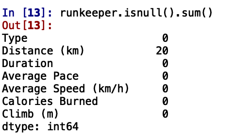
runkeeper.isnull().sum()
👉 There are 20 missing values in the column of 'Distance'. It is mostly because the GPS was not able to detect the location so the distance could not be captured.
As you can see from the last ouput, there are 20 missing values in the column of 'Distance'. I cannot go back in time to get those data but I can fill in the missing values with an average value. This process is called median imputation. When imputing the median to fill in missing data, I need to consider that the distance varies for different activities (e.g., walking vs. running). I will filter the DataFrames by activity type (Type) and calculate each activity's median distance, then fill in the missing values with those median. I choose median because mean is very sensitive to outliers, thus it is more accurate to use median in this case.
##Dealing with missing values for each training activity type (filling with median)
median_running = runkeeper[runkeeper['Type'] == 'Running']['Distance (km)'].median()
median_running #3.5
runkeeper['Distance (km)'].fillna(median_running,inplace=True)

median_walking = runkeeper[runkeeper['Type'] == 'Walking']['Distance (km)'].median()
median_walking #1.62
runkeeper['Distance (km)'].fillna(median_walking,inplace=True)

median_cycling = runkeeper[runkeeper['Type'] == 'Cycling']['Distance (km)'].median()
median_cycling #6.52
runkeeper['Distance (km)'].fillna(median_cycling,inplace=True)

#Check any missing values again
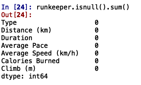
runkeeper.isnull().sum()
👉 All missing values are cleared!
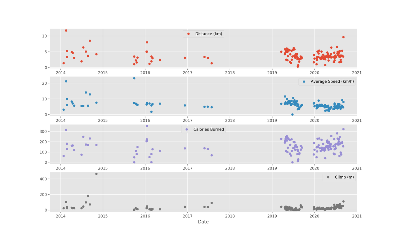
Since most of the activities in my data were 'Running' (143 to be exact), so I will focus on plotting the running metrics.
A good visualization is a figure with 4 subplots, one for each running metric (each numerical column). Each subplot will have a different y - axie, which is explained in each legend. The x axis, 'Date' is hared among all subplots.
# Import matplotlib, set style and ignore warning
import matplotlib.pyplot as plt
%matplotlib inline
import warnings
plt.style.use('ggplot')
warnings.filterwarnings(
    action='ignore', module='matplotlib.figure', category=UserWarning,
    message=('This figure includes Axes that are not compatible with tight_layout, so results might be incorrect.')
)

# Choosing only running for analysis
df_run = runkeeper[runkeeper['Type'] == 'Running'].copy()

#Prepare data subsetiing period from 2014 to 2020
runs_subset_2014_2020 = df_run['2019':'2014']

runs_subset_2014_2020.plot(subplots=True,
                           sharex=False,
                           figsize=(12,16),
                           linestyle='none',
                           marker='o',
                           markersize=5,
                          )

# Show plot
plt.show()
👉 The plot shows that I ran more frequently between the year of 2019 and 2020.
Since I have been running for the past 7 years, I would want to know my overall performance. In this part, I will use resample() to group the time series data by a sampling period and apply several methods to each sampling period (i.e. annually and weekly)
#Prepare data subsetiing period from 2014 to 2020
runs_subset_2014_2020 = df_run['2020':'2014']

#Calculate annual statistics (My average run in last 7 years)
annual_average = runs_subset_2014_2020.resample('A').mean()

#Calculate weekly statistics (My weekly run in last 7 years)
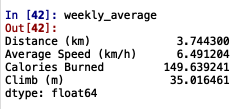
weekly_average = runs_subset_2014_2020.resample('W').mean().mean()

#No. of Training per week I had on average
weekly_counts_average = runs_subset_2014_2020['Distance (km)'].resample('W').count().mean()
weekly_counts_average
👉 There are null numbers in 2018 because there was no activities going on.
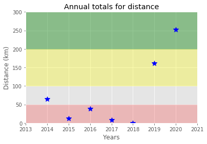
I am always a 'gym' person but I try to exercise outdoor whenever I can. I set a goal to run outdoor at least 3km and twice per week. That will be 6km per week, 24km per month and 288km per year. Let's visualize my annual distance (km) from 2014 to 2020 to see if I reached my goal each year. Only stars in the green region indicate success.
## Did I reach my goals?
# Prepare data
df_run_dist_annual = df_run['2020':'2014']['Distance (km)'].resample('A').sum()

# Create plot
import matplotlib.pyplot as plt
fig = plt.figure(figsize=(10, 5))

# Plot and customize
ax = df_run_dist_annual.plot(marker='*', markersize=10, linewidth=0, color='blue')
ax.set(ylim=[0, 300],
       xlim=['2014','2020'],
       ylabel='Distance (km)',
       xlabel='Years',
       title='Annual totals for distance')

ax.axhspan(1000, 1210, color='green', alpha=0.4)
ax.axhspan(800, 1000, color='yellow', alpha=0.3)
ax.axhspan(0, 800, color='red', alpha=0.2)

# Show plot
plt.show()
👉 I have reached my goal in 2020!
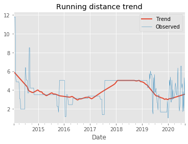
Let's dive a little deeper into the data to answer a difficult question: am I progressing in terms of my running skills?
To answer this question, I will decompose my weekly distance run and visually compare it to the raw data. A red trend line will represent the weekly distance run.
We are going to use statsmodels library to decompose the weekly trend.
##Am I progressing?

# Import required library
import statsmodels.api as sm

# Prepare data
df_run_dist_wkly = df_run['2020':'2014']['Distance (km)'].resample('W').bfill()
df_run_dist_wkly = df_run_dist_wkly.dropna(axis=0)
decomposed = sm.tsa.seasonal_decompose(df_run_dist_wkly, extrapolate_trend=1, period=52)

# Create plot
fig = plt.figure(figsize=(10, 5))

# Plot and customize
ax = decomposed.trend.plot(label='Trend', linewidth=2)
ax = decomposed.observed.plot(label='Observed', linewidth=0.5)

ax.legend()
ax.set_title('Running distance trend')

# Show plot
plt.show()
👉 As you can observe, I progressed more steadily toward the year of 2020.
## Summary Report
# Concatenating three DataFrames
df_walk = runkeeper[runkeeper['Type'] == 'Walking'].copy()
df_cycle = runkeeper[runkeeper['Type'] == 'Cycling'].copy()
df_run_walk_cycle = df_run.append([df_walk, df_cycle]).sort_index(ascending=False)

dist_climb_cols, speed_col = ['Distance (km)', 'Climb (m)'], ['Average Speed (km/h)']

# Calculating total distance and climb in each type of activities
df_totals = df_run_walk_cycle.groupby('Type')[dist_climb_cols].sum()

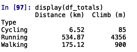
#Totals for different training types:
display(df_totals)
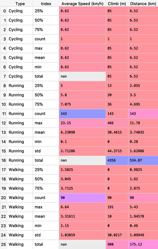
# Calculating summary statistics for each type of activities
df_summary = df_run_walk_cycle.groupby('Type')[dist_climb_cols + speed_col].describe()

# Combine totals with summary
for i in dist_climb_cols:
    df_summary[i, 'total'] = df_totals[i]

print('Summary statistics for different training types:')
df_summary_total = df_summary.stack()
Based on the analysis of my Runkeeper Fitness data, I was very inactive in running outdoor before 2019 so it is reasonable to conclude that I was able to finish my first marathon mainly because of my strength that was built in the gym. Additionally, I discovered an insight from my data which was the increased progression of my running after the marathon. To think of it, the insight makes sense to me because my first marathon was memorable and life-changing. It taught me the lesson of determination and patience. Ever since then, whenever I feel demotivated, I will go out of my house and run as to remind myself that 'life is like a marathon'.
This project is inspired by https://projects.datacamp.com/projects/727


