pip install bokeh-plot
To load this extension in jupyter notebook:
%load_ext bokeh_plot
The following syntax is supported:
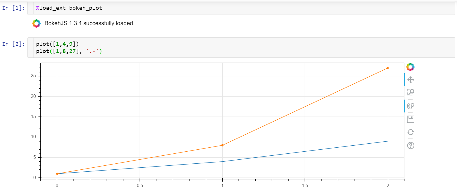
plot([1,4,9])             # x is automatic
plot([1,4,9], '.-')       # line and dots
plot([1,2,3], [1,4,9])    # x and y
plot([1,2,3], [1,4,9], '.-')    # x, y and line style
Several plots in one figure:
Interactive controls:
click and drag = pan
mouse wheel = zoom,
wheel on x axis = scroll horizontally
wheel on y axis = scroll vertically
Multiple plot syntax (equivalent ways to draw it):
x = [1,5,10]
y1 = [1,4,9]
y2 = [1,8,27]

- plot(x, y1, '.-')        # solid line with dots
  plot(x, y2, '.-g')       # the second plot is green

- plot([y1, y2])           # auto x, auto colors

- plot(x, [y1, y2])

- plot([y1, y2], '.-bg')   # blue and green

- plot([y1, y2], style=['.', '.-'], color=['b', 'g'])

- plot(x, y1, '.-', x, y2, '.-g')
The following markers are supported so far:
'.' dots
'-' line
'.-' dots+line
The following colors are supported so far:
'b' blue
'g' green
'r' red
'O' orange  (capital O to avoid clashes with 'o' for open dots)
NB The color specifier must go after the marker if both are present.
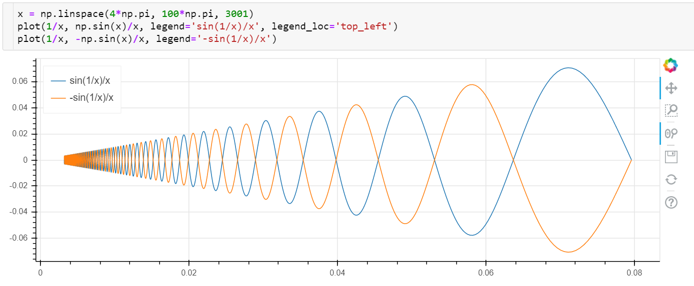
Legend:
- plot([1,2,3], [1,4,9], label='plot1')
  plot([1,2,3], [2,5,10], label='plot2')

- plot([y1, y2], label=['y1', 'y2'])
Legend location:
- plot([1,2,3], [1,4,9], label='plot1', legend_loc='top_left')
  plot([1,2,3], [2,5,10], label='plot2')
Other legend locations: https://docs.bokeh.org/en/latest/docs/user_guide/styling.html#location
Axes labels:
- plot([1,2,3], xlabel='time', ylabel='value')
- xlabel('time'); ylabel('value')
- xylabels('time', 'value')
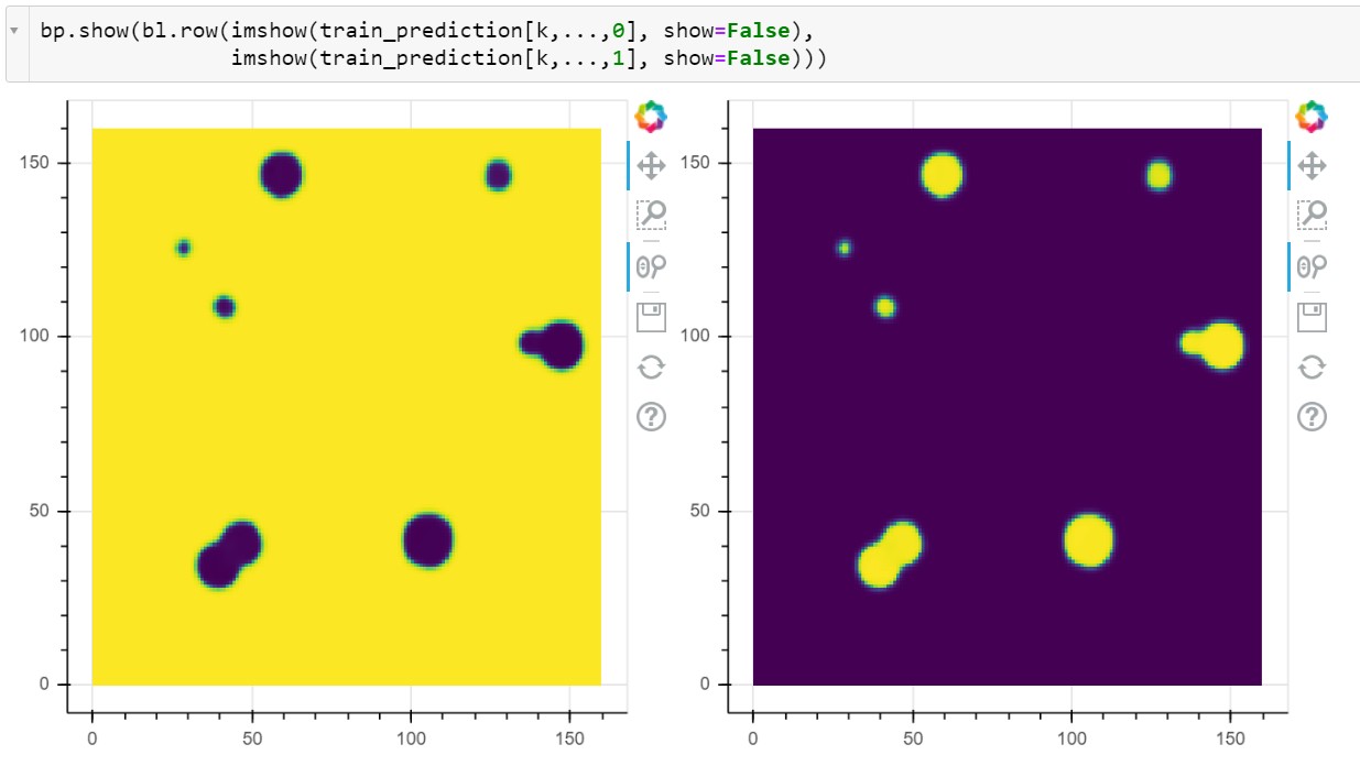
Several images side by side:
- imshow(im1, im2)
All the images are displayed in a row. For more tricky layouts
Here bp stands for bokeh.plot, bl is is a shortcut for bokeh.layouts.
There're three common layouts: bl.row, bl.column and bl.gridplot (the former two accept list of figures,
the latter one accepts a list of lists of figures).
Other uses:
-
semilogx(),semilogy()andloglog()show (semi)logarithmic plots with the same syntax asplot(). -
hist(x)displays a histogram of x -
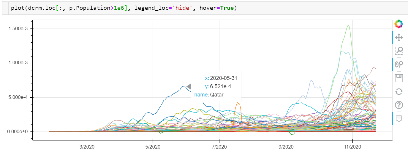
plot(x, y, hover=True)displays point coordinates on mouse hover. -
plot(x, y, vline=1, hline=1.5, vline_color='red')in addition to the (x, y) plot displays an infinite vertical line with x=1 and custom red color and an infinite horizontal line with y=1.5 and the default pink color. -
plot(df)plots all columns of the dataframe as separate lines on the same figure with column names displayed in the legend and with index taken as the x axis values. If the legend grows too long, it can be hidden withlegend_loc='hide'(new in v0.1.13):
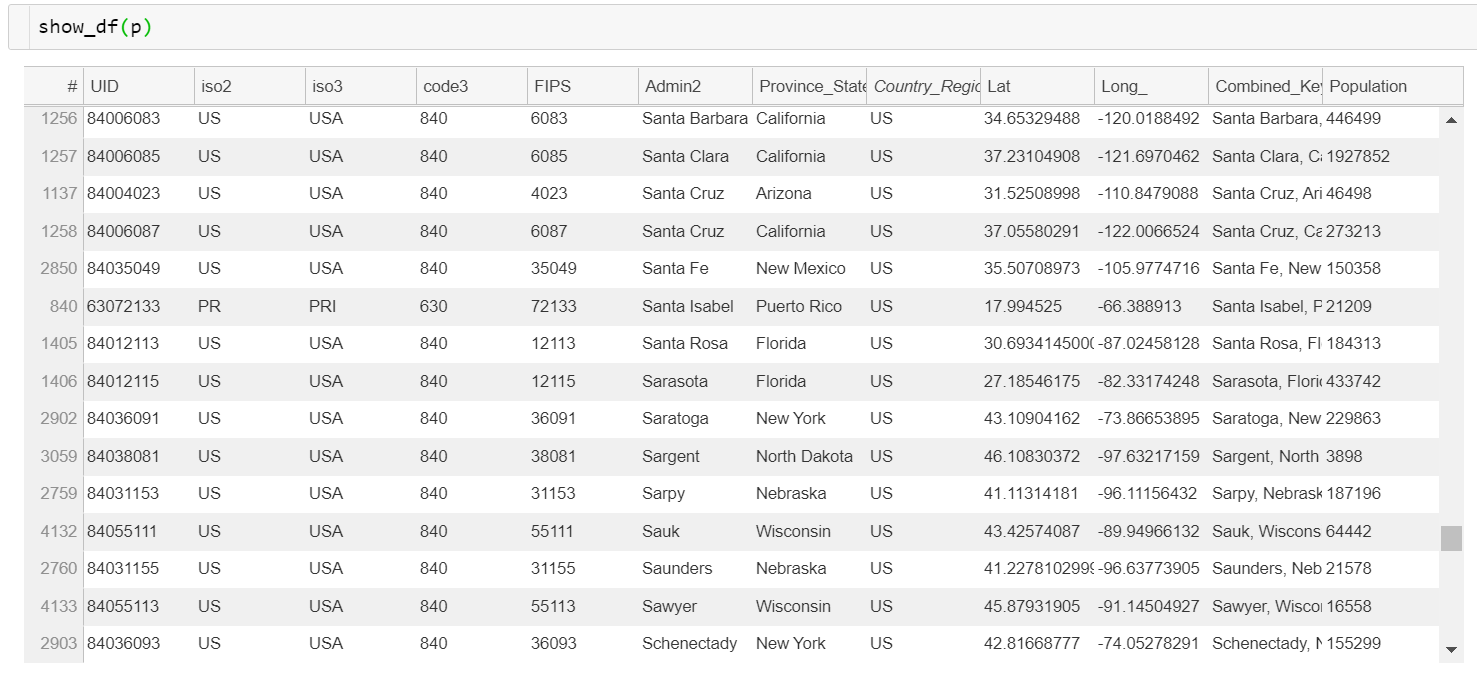
show_df(df)displays pandas dataframe as a table (new in v0.1.14):
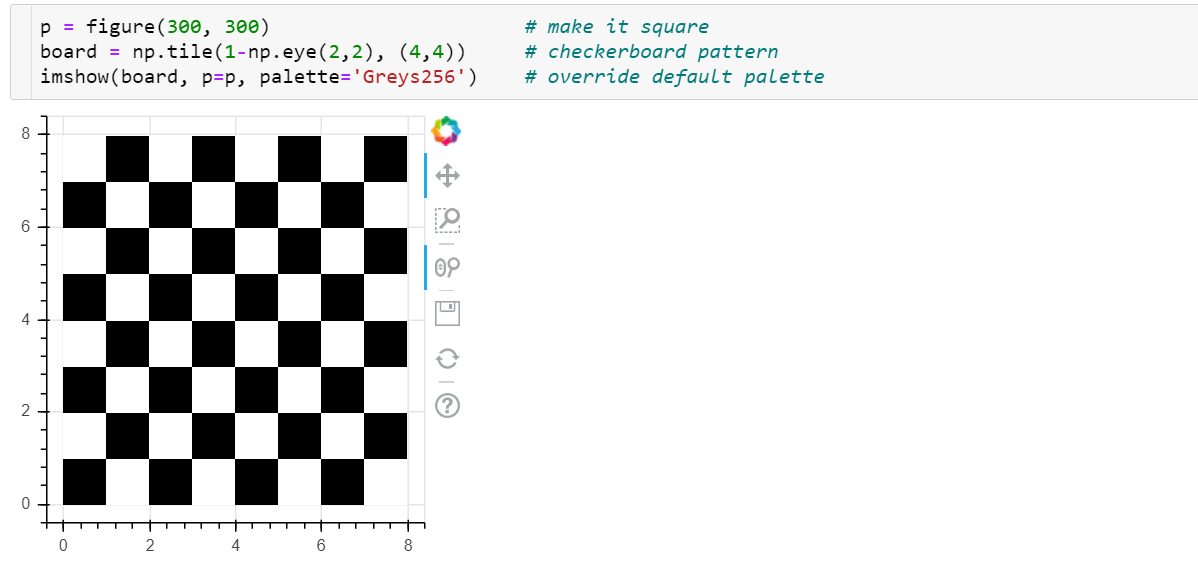
imshow(a)displays an array as an image:
Complete list of palettes: https://docs.bokeh.org/en/latest/docs/reference/palettes.html
See also a contour plot example in the bokeh gallery page
bokeh-plot is a thin wrapper over the excellent bokeh library that cuts down the amount of boilerplate code.
The following two cells are equivalent:
